1 Introduction
You’re reading the first edition of R4DS; for the latest on this topic see the Introduction chapter in the second edition.
Data science is an exciting discipline that allows you to turn raw data into understanding, insight, and knowledge. The goal of “R for Data Science” is to help you learn the most important tools in R that will allow you to do data science. After reading this book, you’ll have the tools to tackle a wide variety of data science challenges, using the best parts of R.
1.1 What you will learn
Data science is a huge field, and there’s no way you can master it by reading a single book. The goal of this book is to give you a solid foundation in the most important tools. Our model of the tools needed in a typical data science project looks something like this:
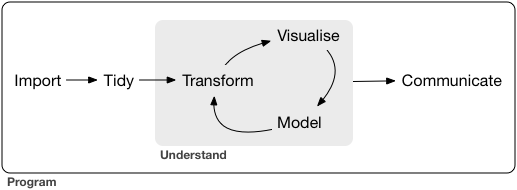
First you must import your data into R. This typically means that you take data stored in a file, database, or web application programming interface (API), and load it into a data frame in R. If you can’t get your data into R, you can’t do data science on it!
Once you’ve imported your data, it is a good idea to tidy it. Tidying your data means storing it in a consistent form that matches the semantics of the dataset with the way it is stored. In brief, when your data is tidy, each column is a variable, and each row is an observation. Tidy data is important because the consistent structure lets you focus your struggle on questions about the data, not fighting to get the data into the right form for different functions.
Once you have tidy data, a common first step is to transform it. Transformation includes narrowing in on observations of interest (like all people in one city, or all data from the last year), creating new variables that are functions of existing variables (like computing speed from distance and time), and calculating a set of summary statistics (like counts or means). Together, tidying and transforming are called wrangling, because getting your data in a form that’s natural to work with often feels like a fight!
Once you have tidy data with the variables you need, there are two main engines of knowledge generation: visualisation and modelling. These have complementary strengths and weaknesses so any real analysis will iterate between them many times.
Visualisation is a fundamentally human activity. A good visualisation will show you things that you did not expect, or raise new questions about the data. A good visualisation might also hint that you’re asking the wrong question, or you need to collect different data. Visualisations can surprise you, but don’t scale particularly well because they require a human to interpret them.
Models are complementary tools to visualisation. Once you have made your questions sufficiently precise, you can use a model to answer them. Models are a fundamentally mathematical or computational tool, so they generally scale well. Even when they don’t, it’s usually cheaper to buy more computers than it is to buy more brains! But every model makes assumptions, and by its very nature a model cannot question its own assumptions. That means a model cannot fundamentally surprise you.
The last step of data science is communication, an absolutely critical part of any data analysis project. It doesn’t matter how well your models and visualisation have led you to understand the data unless you can also communicate your results to others.
Surrounding all these tools is programming. Programming is a cross-cutting tool that you use in every part of the project. You don’t need to be an expert programmer to be a data scientist, but learning more about programming pays off because becoming a better programmer allows you to automate common tasks, and solve new problems with greater ease.
You’ll use these tools in every data science project, but for most projects they’re not enough. There’s a rough 80-20 rule at play; you can tackle about 80% of every project using the tools that you’ll learn in this book, but you’ll need other tools to tackle the remaining 20%. Throughout this book we’ll point you to resources where you can learn more.
1.2 How this book is organised
The previous description of the tools of data science is organised roughly according to the order in which you use them in an analysis (although of course you’ll iterate through them multiple times). In our experience, however, this is not the best way to learn them:
Starting with data ingest and tidying is sub-optimal because 80% of the time it’s routine and boring, and the other 20% of the time it’s weird and frustrating. That’s a bad place to start learning a new subject! Instead, we’ll start with visualisation and transformation of data that’s already been imported and tidied. That way, when you ingest and tidy your own data, your motivation will stay high because you know the pain is worth it.
Some topics are best explained with other tools. For example, we believe that it’s easier to understand how models work if you already know about visualisation, tidy data, and programming.
Programming tools are not necessarily interesting in their own right, but do allow you to tackle considerably more challenging problems. We’ll give you a selection of programming tools in the middle of the book, and then you’ll see how they can combine with the data science tools to tackle interesting modelling problems.
Within each chapter, we try and stick to a similar pattern: start with some motivating examples so you can see the bigger picture, and then dive into the details. Each section of the book is paired with exercises to help you practice what you’ve learned. While it’s tempting to skip the exercises, there’s no better way to learn than practicing on real problems.
1.3 What you won’t learn
There are some important topics that this book doesn’t cover. We believe it’s important to stay ruthlessly focused on the essentials so you can get up and running as quickly as possible. That means this book can’t cover every important topic.
1.3.1 Big data
This book proudly focuses on small, in-memory datasets. This is the right place to start because you can’t tackle big data unless you have experience with small data. The tools you learn in this book will easily handle hundreds of megabytes of data, and with a little care you can typically use them to work with 1-2 Gb of data. If you’re routinely working with larger data (10-100 Gb, say), you should learn more about data.table. This book doesn’t teach data.table because it has a very concise interface which makes it harder to learn since it offers fewer linguistic cues. But if you’re working with large data, the performance payoff is worth the extra effort required to learn it.
If your data is bigger than this, carefully consider if your big data problem might actually be a small data problem in disguise. While the complete data might be big, often the data needed to answer a specific question is small. You might be able to find a subset, subsample, or summary that fits in memory and still allows you to answer the question that you’re interested in. The challenge here is finding the right small data, which often requires a lot of iteration.
Another possibility is that your big data problem is actually a large number of small data problems. Each individual problem might fit in memory, but you have millions of them. For example, you might want to fit a model to each person in your dataset. That would be trivial if you had just 10 or 100 people, but instead you have a million. Fortunately each problem is independent of the others (a setup that is sometimes called embarrassingly parallel), so you just need a system (like Hadoop or Spark) that allows you to send different datasets to different computers for processing. Once you’ve figured out how to answer the question for a single subset using the tools described in this book, you learn new tools like sparklyr, rhipe, and ddr to solve it for the full dataset.
1.3.2 Python, Julia, and friends
In this book, you won’t learn anything about Python, Julia, or any other programming language useful for data science. This isn’t because we think these tools are bad. They’re not! And in practice, most data science teams use a mix of languages, often at least R and Python.
However, we strongly believe that it’s best to master one tool at a time. You will get better faster if you dive deep, rather than spreading yourself thinly over many topics. This doesn’t mean you should only know one thing, just that you’ll generally learn faster if you stick to one thing at a time. You should strive to learn new things throughout your career, but make sure your understanding is solid before you move on to the next interesting thing.
We think R is a great place to start your data science journey because it is an environment designed from the ground up to support data science. R is not just a programming language, but it is also an interactive environment for doing data science. To support interaction, R is a much more flexible language than many of its peers. This flexibility comes with its downsides, but the big upside is how easy it is to evolve tailored grammars for specific parts of the data science process. These mini languages help you think about problems as a data scientist, while supporting fluent interaction between your brain and the computer.
1.3.3 Non-rectangular data
This book focuses exclusively on rectangular data: collections of values that are each associated with a variable and an observation. There are lots of datasets that do not naturally fit in this paradigm, including images, sounds, trees, and text. But rectangular data frames are extremely common in science and industry, and we believe that they are a great place to start your data science journey.
1.3.4 Hypothesis confirmation
It’s possible to divide data analysis into two camps: hypothesis generation and hypothesis confirmation (sometimes called confirmatory analysis). The focus of this book is unabashedly on hypothesis generation, or data exploration. Here you’ll look deeply at the data and, in combination with your subject knowledge, generate many interesting hypotheses to help explain why the data behaves the way it does. You evaluate the hypotheses informally, using your scepticism to challenge the data in multiple ways.
The complement of hypothesis generation is hypothesis confirmation. Hypothesis confirmation is hard for two reasons:
You need a precise mathematical model in order to generate falsifiable predictions. This often requires considerable statistical sophistication.
You can only use an observation once to confirm a hypothesis. As soon as you use it more than once you’re back to doing exploratory analysis. This means to do hypothesis confirmation you need to “preregister” (write out in advance) your analysis plan, and not deviate from it even when you have seen the data. We’ll talk a little about some strategies you can use to make this easier in modelling.
It’s common to think about modelling as a tool for hypothesis confirmation, and visualisation as a tool for hypothesis generation. But that’s a false dichotomy: models are often used for exploration, and with a little care you can use visualisation for confirmation. The key difference is how often do you look at each observation: if you look only once, it’s confirmation; if you look more than once, it’s exploration.
1.4 Prerequisites
We’ve made a few assumptions about what you already know in order to get the most out of this book. You should be generally numerically literate, and it’s helpful if you have some programming experience already. If you’ve never programmed before, you might find Hands on Programming with R by Garrett to be a useful adjunct to this book.
There are four things you need to run the code in this book: R, RStudio, a collection of R packages called the tidyverse, and a handful of other packages. Packages are the fundamental units of reproducible R code. They include reusable functions, the documentation that describes how to use them, and sample data.
1.4.1 R
To download R, go to CRAN, the comprehensive R archive network. CRAN is composed of a set of mirror servers distributed around the world and is used to distribute R and R packages. Don’t try and pick a mirror that’s close to you: instead use the cloud mirror, https://cloud.r-project.org, which automatically figures it out for you.
A new major version of R comes out once a year, and there are 2-3 minor releases each year. It’s a good idea to update regularly. Upgrading can be a bit of a hassle, especially for major versions, which require you to reinstall all your packages, but putting it off only makes it worse.
1.4.2 RStudio
RStudio is an integrated development environment, or IDE, for R programming. Download and install it from http://www.rstudio.com/download. RStudio is updated a couple of times a year. When a new version is available, RStudio will let you know. It’s a good idea to upgrade regularly so you can take advantage of the latest and greatest features. For this book, make sure you have at least RStudio 1.0.0.
When you start RStudio, you’ll see two key regions in the interface:
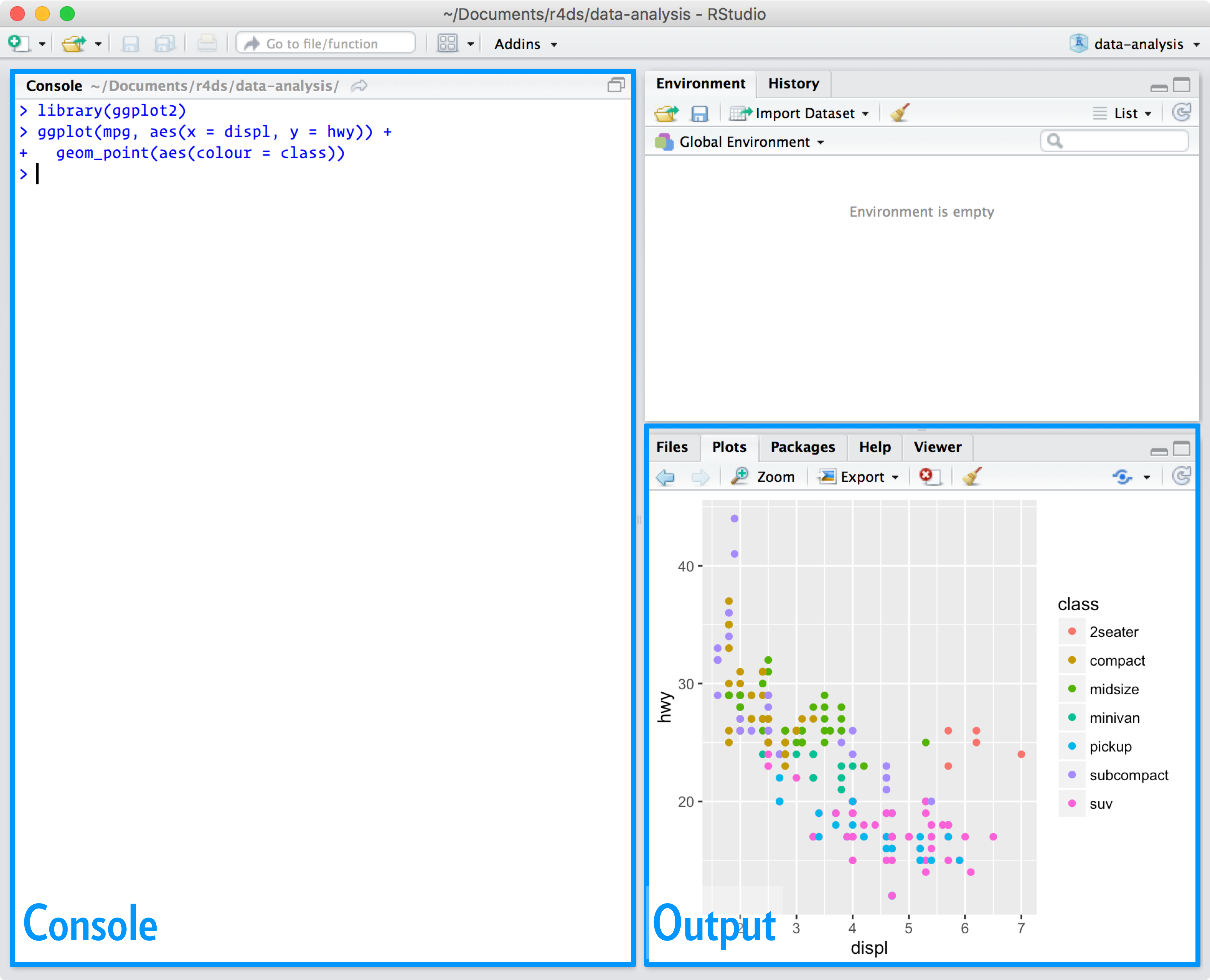
For now, all you need to know is that you type R code in the console pane, and press enter to run it. You’ll learn more as we go along!
1.4.3 The tidyverse
You’ll also need to install some R packages. An R package is a collection of functions, data, and documentation that extends the capabilities of base R. Using packages is key to the successful use of R. The majority of the packages that you will learn in this book are part of the so-called tidyverse. The packages in the tidyverse share a common philosophy of data and R programming, and are designed to work together naturally.
You can install the complete tidyverse with a single line of code:
install.packages("tidyverse")On your own computer, type that line of code in the console, and then press enter to run it. R will download the packages from CRAN and install them on to your computer. If you have problems installing, make sure that you are connected to the internet, and that https://cloud.r-project.org/ isn’t blocked by your firewall or proxy.
You will not be able to use the functions, objects, and help files in a package until you load it with library(). Once you have installed a package, you can load it with the library() function:
library(tidyverse)
#> ── Attaching core tidyverse packages ──────────────────────── tidyverse 2.0.0 ──
#> ✔ dplyr     1.1.4     ✔ readr     2.1.5
#> ✔ forcats   1.0.0     ✔ stringr   1.5.1
#> ✔ ggplot2   3.5.1     ✔ tibble    3.2.1
#> ✔ lubridate 1.9.4     ✔ tidyr     1.3.1
#> ✔ purrr     1.0.4
#> ── Conflicts ────────────────────────────────────────── tidyverse_conflicts() ──
#> ✖ dplyr::filter() masks stats::filter()
#> ✖ dplyr::lag()    masks stats::lag()
#> ℹ Use the conflicted package (<http://conflicted.r-lib.org/>) to force all conflicts to become errors
This tells you that tidyverse is loading the ggplot2, tibble, tidyr, readr, purrr, and dplyr packages. These are considered to be the core of the tidyverse because you’ll use them in almost every analysis.
Packages in the tidyverse change fairly frequently. You can see if updates are available, and optionally install them, by running tidyverse_update().
1.4.4 Other packages
There are many other excellent packages that are not part of the tidyverse, because they solve problems in a different domain, or are designed with a different set of underlying principles. This doesn’t make them better or worse, just different. In other words, the complement to the tidyverse is not the messyverse, but many other universes of interrelated packages. As you tackle more data science projects with R, you’ll learn new packages and new ways of thinking about data.
In this book we’ll use three data packages from outside the tidyverse:
install.packages(c("nycflights13", "gapminder", "Lahman"))These packages provide data on airline flights, world development, and baseball that we’ll use to illustrate key data science ideas.
1.5 Running R code
The previous section showed you a couple of examples of running R code. Code in the book looks like this:
1 + 2
#> [1] 3
If you run the same code in your local console, it will look like this:
> 1 + 2
[1] 3
There are two main differences. In your console, you type after the >, called the prompt; we don’t show the prompt in the book. In the book, output is commented out with #>; in your console it appears directly after your code. These two differences mean that if you’re working with an electronic version of the book, you can easily copy code out of the book and into the console.
Throughout the book we use a consistent set of conventions to refer to code:
Functions are in a code font and followed by parentheses, like
sum(), ormean().Other R objects (like data or function arguments) are in a code font, without parentheses, like
flightsorx.If we want to make it clear what package an object comes from, we’ll use the package name followed by two colons, like
dplyr::mutate(), ornycflights13::flights. This is also valid R code.
1.6 Getting help and learning more
This book is not an island; there is no single resource that will allow you to master R. As you start to apply the techniques described in this book to your own data you will soon find questions that we do not answer. This section describes a few tips on how to get help, and to help you keep learning.
If you get stuck, start with Google. Typically adding “R” to a query is enough to restrict it to relevant results: if the search isn’t useful, it often means that there aren’t any R-specific results available. Google is particularly useful for error messages. If you get an error message and you have no idea what it means, try googling it! Chances are that someone else has been confused by it in the past, and there will be help somewhere on the web. (If the error message isn’t in English, run Sys.setenv(LANGUAGE = "en") and re-run the code; you’re more likely to find help for English error messages.)
If Google doesn’t help, try stackoverflow. Start by spending a little time searching for an existing answer, including [R] to restrict your search to questions and answers that use R. If you don’t find anything useful, prepare a minimal reproducible example or reprex. A good reprex makes it easier for other people to help you, and often you’ll figure out the problem yourself in the course of making it.
There are three things you need to include to make your example reproducible: required packages, data, and code.
Packages should be loaded at the top of the script, so it’s easy to see which ones the example needs. This is a good time to check that you’re using the latest version of each package; it’s possible you’ve discovered a bug that’s been fixed since you installed the package. For packages in the tidyverse, the easiest way to check is to run
tidyverse_update().-
The easiest way to include data in a question is to use
dput()to generate the R code to recreate it. For example, to recreate themtcarsdataset in R, I’d perform the following steps:- Run
dput(mtcars)in R - Copy the output
- In my reproducible script, type
mtcars <-then paste.
Try and find the smallest subset of your data that still reveals the problem.
- Run
-
Spend a little bit of time ensuring that your code is easy for others to read:
Make sure you’ve used spaces and your variable names are concise, yet informative.
Use comments to indicate where your problem lies.
Do your best to remove everything that is not related to the problem.
The shorter your code is, the easier it is to understand, and the easier it is to fix.
Finish by checking that you have actually made a reproducible example by starting a fresh R session and copying and pasting your script in.
You should also spend some time preparing yourself to solve problems before they occur. Investing a little time in learning R each day will pay off handsomely in the long run. One way is to follow what Hadley, Garrett, and everyone else at RStudio are doing on the RStudio blog. This is where we post announcements about new packages, new IDE features, and in-person courses. You might also want to follow Hadley (@hadleywickham) or Garrett (@statgarrett) on Twitter, or follow @rstudiotips to keep up with new features in the IDE.
To keep up with the R community more broadly, we recommend reading http://www.r-bloggers.com: it aggregates over 500 blogs about R from around the world. If you’re an active Twitter user, follow the (#rstats) hashtag. Twitter is one of the key tools that Hadley uses to keep up with new developments in the community.
1.7 Acknowledgements
This book isn’t just the product of Hadley and Garrett, but is the result of many conversations (in person and online) that we’ve had with the many people in the R community. There are a few people we’d like to thank in particular, because they have spent many hours answering our dumb questions and helping us to better think about data science:
Jenny Bryan and Lionel Henry for many helpful discussions around working with lists and list-columns.
The three chapters on workflow were adapted (with permission), from http://stat545.com/block002_hello-r-workspace-wd-project.html by Jenny Bryan.
Genevera Allen for discussions about models, modelling, the statistical learning perspective, and the difference between hypothesis generation and hypothesis confirmation.
Yihui Xie for his work on the bookdown package, and for tirelessly responding to my feature requests.
Bill Behrman for his thoughtful reading of the entire book, and for trying it out with his data science class at Stanford.
The #rstats twitter community who reviewed all of the draft chapters and provided tons of useful feedback.
Tal Galili for augmenting his dendextend package to support a section on clustering that did not make it into the final draft.
This book was written in the open, and many people contributed pull requests to fix minor problems. Special thanks goes to everyone who contributed via GitHub:
Thanks go to all contributers in alphabetical order: A. s, Abhinav Singh, Ahmed ElGabbas, Ajay Deonarine, @AlanFeder, Albert Y. Kim, @Alex, Andrea Gilardi, Andrew Landgraf, Angela Li, Azza Ahmed, Ben Herbertson, Ben Marwick, Ben Steinberg, Benjamin Yeh, Bianca Peterson, Bill Behrman, @BirgerNi, Brandon Greenwell, Brent Brewington, Brett Klamer, Brian G. Barkley, Charlotte Wickham, Christian G. Warden, Christian Heinrich, Christian Mongeau, Colin Gillespie, Cooper Morris, Curtis Alexander, @DSGeoff, Daniel Gromer, David Clark, David Rubinger, Derwin McGeary, Devin Pastoor, Dirk Eddelbuettel, Dylan Cashman, Earl Brown, Edwin Thoen, Eric Watt, Erik Erhardt, Etienne B. Racine, Everett Robinson, Flemming Villalona, Floris Vanderhaeghe, Garrick Aden-Buie, George Wang, Gregory Jefferis, Gustav W Delius, Hao Chen, Hengni Cai, Hiroaki Yutani, Hojjat Salmasian, Ian Lyttle, Ian Sealy, Ivan Krukov, Jacek Kolacz, Jacob Kaplan, Jakub Nowosad, Jazz Weisman, Jeff Boichuk, Jeffrey Arnold, Jen Ren, Jennifer (Jenny) Bryan, Jeroen Janssens, Jim Hester, Joanne Jang, Johannes Gruber, John Blischak, John D. Storey, John Sears, Jon Calder, @Jonas, Jonathan Page, Jose Roberto Ayala Solares, Josh Goldberg, Julia Stewart Lowndes, Julian During, Justinas Petuchovas, Kara Woo, Kara de la Marck, Katrin Leinweber, Kenny Darrell, Kirill Müller, Kirill Sevastyanenko, Kunal Marwaha, @KyleHumphrey, Lawrence Wu, Luke Smith, Luke W Johnston, @MJMarshall, Mara Averick, Maria Paula Caldas, Mark Beveridge, Matt Herman, @MattWittbrodt, Matthew Hendrickson, Matthew Sedaghatfar, Mauro Lepore, Michael Henry, Mine Cetinkaya-Rundel, Mustafa Ascha, Nelson Areal, Nicholas Tierney, Nick Clark, Nina Munkholt Jakobsen, Nirmal Patel, Nischal Shrestha, Noah Landesberg, @OaCantona, Pablo E, Patrick Kennedy, @Paul, Peter Hurford, Rademeyer Vermaak, Radu Grosu, Ranae Dietzel, Riva Quiroga, Rob Tenorio, Robert Schuessler, Robin Gertenbach, Rohan Alexander, @RomeroBarata, S’busiso Mkhondwane, @Saghir, Sam Firke, Seamus McKinsey, Sebastian Kraus, Shannon Ellis, @Sophiazj, Steve Mortimer, Stéphane Guillou, TJ Mahr, Tal Galili, Terence Teo, Thomas Klebel, Tim Waterhouse, Tom Prior, Ulrik Lyngs, Will Beasley, Yihui Xie, Yiming (Paul) Li, Yu Yu Aung, Zach Bogart, Zhuoer Dong, @a-rosenberg, adi pradhan, @andrewmacfarland, bahadir cankardes, @batpigandme, @behrman, @boardtc, @djbirke, @harrismcgehee, @jennybc, @jjchern, @jonathanflint, @juandering, @kaetschap, @kdpsingh, @koalabearski, @lindbrook, @nate-d-olson, @nattalides, @nickelas, @nwaff, @pete, @rlzijdeman, @robertchu03, @robinlovelace, @robinsones, @seamus-mckinsey, @seanpwilliams, @shoili, @sibusiso16, @spirgel, @svenski, @twgardner2, @yahwes, @zeal626, @蒋雨蒙.
1.8 Colophon
An online version of this book is available at http://r4ds.had.co.nz. It will continue to evolve in between reprints of the physical book. The source of the book is available at https://github.com/hadley/r4ds. The book is powered by https://bookdown.org which makes it easy to turn R markdown files into HTML, PDF, and EPUB.
This book was built with:
sessioninfo::session_info(c("tidyverse"))
#> ─ Session info ───────────────────────────────────────────────────────────────
#>  setting  value
#>  version  R version 4.4.2 (2024-10-31)
#>  os       Ubuntu 24.04.1 LTS
#>  system   x86_64, linux-gnu
#>  ui       X11
#>  language (EN)
#>  collate  C.UTF-8
#>  ctype    C.UTF-8
#>  tz       UTC
#>  date     2025-02-18
#>  pandoc   3.1.11 @ /opt/hostedtoolcache/pandoc/3.1.11/x64/ (via rmarkdown)
#>  quarto   NA
#>
#> ─ Packages ───────────────────────────────────────────────────────────────────
#>  ! package       * version date (UTC) lib source
#>    askpass         1.2.1   2024-10-04 [1] RSPM
#>    backports       1.5.0   2024-05-23 [1] RSPM
#>    base64enc       0.1-3   2015-07-28 [1] RSPM
#>    bit             4.5.0.1 2024-12-03 [1] RSPM
#>    bit64           4.6.0-1 2025-01-16 [1] RSPM
#>    blob            1.2.4   2023-03-17 [1] RSPM
#>    broom           1.0.7   2024-09-26 [1] RSPM
#>    bslib           0.9.0   2025-01-30 [1] RSPM
#>    cachem          1.1.0   2024-05-16 [1] RSPM
#>    callr           3.7.6   2024-03-25 [1] RSPM
#>    cellranger      1.1.0   2016-07-27 [1] RSPM
#>    cli             3.6.4   2025-02-13 [1] RSPM
#>    clipr           0.8.0   2022-02-22 [1] RSPM
#>    colorspace      2.1-1   2024-07-26 [1] RSPM
#>    conflicted      1.2.0   2023-02-01 [1] RSPM
#>  R cpp11           <NA>    <NA>       [?] <NA>
#>    crayon          1.5.3   2024-06-20 [1] RSPM
#>    curl            6.2.0   2025-01-23 [1] RSPM
#>    data.table      1.16.4  2024-12-06 [1] RSPM
#>    DBI             1.2.3   2024-06-02 [1] RSPM
#>    dbplyr          2.5.0   2024-03-19 [1] RSPM
#>    digest          0.6.37  2024-08-19 [1] RSPM
#>    dplyr         * 1.1.4   2023-11-17 [1] RSPM
#>    dtplyr          1.3.1   2023-03-22 [1] RSPM
#>    evaluate        1.0.3   2025-01-10 [1] RSPM
#>    fansi           1.0.6   2023-12-08 [1] RSPM
#>    farver          2.1.2   2024-05-13 [1] RSPM
#>    fastmap         1.2.0   2024-05-15 [1] RSPM
#>    fontawesome     0.5.3   2024-11-16 [1] RSPM
#>    forcats       * 1.0.0   2023-01-29 [1] RSPM
#>    fs              1.6.5   2024-10-30 [1] RSPM
#>    gargle          1.5.2   2023-07-20 [1] RSPM
#>    generics        0.1.3   2022-07-05 [1] RSPM
#>    ggplot2       * 3.5.1   2024-04-23 [1] RSPM
#>    glue            1.8.0   2024-09-30 [1] RSPM
#>    googledrive     2.1.1   2023-06-11 [1] RSPM
#>    googlesheets4   1.1.1   2023-06-11 [1] RSPM
#>    gtable          0.3.6   2024-10-25 [1] RSPM
#>    haven           2.5.4   2023-11-30 [1] RSPM
#>    highr           0.11    2024-05-26 [1] RSPM
#>    hms             1.1.3   2023-03-21 [1] RSPM
#>    htmltools       0.5.8.1 2024-04-04 [1] RSPM
#>    httr            1.4.7   2023-08-15 [1] RSPM
#>    ids             1.0.1   2017-05-31 [1] RSPM
#>    isoband         0.2.7   2022-12-20 [1] RSPM
#>    jquerylib       0.1.4   2021-04-26 [1] RSPM
#>    jsonlite        1.8.9   2024-09-20 [1] RSPM
#>    knitr           1.49    2024-11-08 [1] RSPM
#>    labeling        0.4.3   2023-08-29 [1] RSPM
#>    lattice         0.22-6  2024-03-20 [3] CRAN (R 4.4.2)
#>    lifecycle       1.0.4   2023-11-07 [1] RSPM
#>    lubridate     * 1.9.4   2024-12-08 [1] RSPM
#>    magrittr        2.0.3   2022-03-30 [1] RSPM
#>    MASS            7.3-61  2024-06-13 [3] CRAN (R 4.4.2)
#>    Matrix          1.7-1   2024-10-18 [3] CRAN (R 4.4.2)
#>    memoise         2.0.1   2021-11-26 [1] RSPM
#>    mgcv            1.9-1   2023-12-21 [3] CRAN (R 4.4.2)
#>    mime            0.12    2021-09-28 [1] RSPM
#>    modelr          0.1.11  2023-03-22 [1] RSPM
#>    munsell         0.5.1   2024-04-01 [1] RSPM
#>    nlme            3.1-166 2024-08-14 [3] CRAN (R 4.4.2)
#>    openssl         2.3.2   2025-02-03 [1] RSPM
#>    pillar          1.10.1  2025-01-07 [1] RSPM
#>    pkgconfig       2.0.3   2019-09-22 [1] RSPM
#>    processx        3.8.5   2025-01-08 [1] RSPM
#>  R progress        <NA>    <NA>       [?] <NA>
#>    ps              1.8.1   2024-10-28 [1] RSPM
#>    purrr         * 1.0.4   2025-02-05 [1] RSPM
#>    R6              2.6.1   2025-02-15 [1] RSPM
#>    ragg            1.3.3   2024-09-11 [1] RSPM
#>    rappdirs        0.3.3   2021-01-31 [1] RSPM
#>    RColorBrewer    1.1-3   2022-04-03 [1] RSPM
#>    readr         * 2.1.5   2024-01-10 [1] RSPM
#>    readxl          1.4.3   2023-07-06 [1] RSPM
#>    rematch         2.0.0   2023-08-30 [1] RSPM
#>    rematch2        2.1.2   2020-05-01 [1] RSPM
#>    reprex          2.1.1   2024-07-06 [1] RSPM
#>    rlang           1.1.5   2025-01-17 [1] RSPM
#>    rmarkdown       2.29    2024-11-04 [1] RSPM
#>    rstudioapi      0.17.1  2024-10-22 [1] RSPM
#>    rvest           1.0.4   2024-02-12 [1] RSPM
#>    sass            0.4.9   2024-03-15 [1] RSPM
#>    scales          1.3.0   2023-11-28 [1] RSPM
#>    selectr         0.4-2   2019-11-20 [1] RSPM
#>    stringi         1.8.4   2024-05-06 [1] RSPM
#>    stringr       * 1.5.1   2023-11-14 [1] RSPM
#>    sys             3.4.3   2024-10-04 [1] RSPM
#>    systemfonts     1.2.1   2025-01-20 [1] RSPM
#>    textshaping     1.0.0   2025-01-20 [1] RSPM
#>    tibble        * 3.2.1   2023-03-20 [1] RSPM
#>    tidyr         * 1.3.1   2024-01-24 [1] RSPM
#>    tidyselect      1.2.1   2024-03-11 [1] RSPM
#>    tidyverse     * 2.0.0   2023-02-22 [1] RSPM
#>    timechange      0.3.0   2024-01-18 [1] RSPM
#>    tinytex         0.54    2024-11-01 [1] RSPM
#>    tzdb            0.4.0   2023-05-12 [1] RSPM
#>    utf8            1.2.4   2023-10-22 [1] RSPM
#>    uuid            1.2-1   2024-07-29 [1] RSPM
#>    vctrs           0.6.5   2023-12-01 [1] RSPM
#>    viridisLite     0.4.2   2023-05-02 [1] RSPM
#>    vroom           1.6.5   2023-12-05 [1] RSPM
#>    withr           3.0.2   2024-10-28 [1] RSPM
#>    xfun            0.50    2025-01-07 [1] RSPM
#>    xml2            1.3.6   2023-12-04 [1] RSPM
#>    yaml            2.3.10  2024-07-26 [1] RSPM
#>
#>  [1] /home/runner/work/_temp/Library
#>  [2] /opt/R/4.4.2/lib/R/site-library
#>  [3] /opt/R/4.4.2/lib/R/library
#>
#>  * ── Packages attached to the search path.
#>  R ── Package was removed from disk.
#>
#> ──────────────────────────────────────────────────────────────────────────────